The Wrong Crowd: What Subway Data Can Tell Us About a Packed Platform

If you arrived at a subway station hoping to board a train as soon as possible, how crowded would you want it to be?

Most people to whom I’ve recently asked this question shared the same hypothesis that I’ve reached after years of taking the New York City subway. You don’t want to arrive to an empty platform, because that implies a train has just left and another one is not imminent. Rather, the more people you see, the longer it’s likely been since the previous train and the less time remains until the next one.

However, too large of a crowd might indicate that the subway system is in an unusual state of heavy delay that’s subject to longer, less predictable intervals between trains. Another way of thinking of this idea is that the relationship between platform crowdedness and expected wait time is non-linear and potentially even U-shaped: at some point, marginally more people implies longer wait times and not shorter ones. You stop “earning” time with more passengers and start actually giving it back.

The shared beliefs of a grumpy mob of commuters doesn’t exactly qualify as legitimate proof of this theory, though. So I tried to substantiate the claim using the time-stamped data that the MTA publishes for all of their trips. The data isn’t perfect and requires a lot of cleaning and a little bit of faith, but it seemed good enough to capture essential patterns. Here’s a daily course of 4-trains originating at Utica Avenue in Brooklyn, traversing the length of Manhattan, and terminating deep in the Bronx:

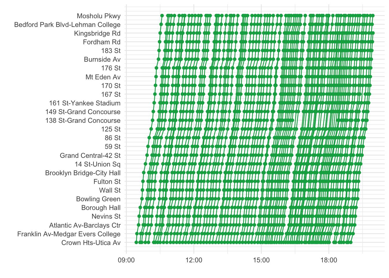
The horizontal distances between adjacent threads at each of the stops listed are equivalent to the wait times between trains. Thankfully they look pretty consistent, besides for a period starting in the late afternoon at 138th Street where it looks like service was suspended for a few hours.

If you apply this logic at scale to each train line, station, direction of travel, and hour of the day, you get a sense of the distribution of wait times that individual commuters experience. Visualized below are some of the busiest stations during rush hour on week days:

You’ll notice a few prominent features of these histograms. Most of them have single peaks somewhere between 2 and 4 minutes – these are the most likely delays, but the average is dragged up in each instance by the characteristic right skew of a non-negative variable. It looks like the MTA can achieve much more consistent departures at points of origin like the express 7 at Hudson Yards or the shuttle at Times Square.

What these histograms don’t demonstrate are exceedingly long tails or even a second, smaller mode somewhere further down the X-axis, which I would think is required to observe the proposed U-shape between platform crowdedness and length of delay. In other words, in most cases I don’t think that there are enough major delays to validate our hypothesis.

But that’s certainly not always the case. Check out the distribution of wait times at 7th Avenue in midtown for downtown B trains on weekday evenings. There is a small but noticeable mini-peak – in this scenario you’re more likely to wait for 15 minutes than you are for 14, and as likely to wait for 18 as you are for 13:

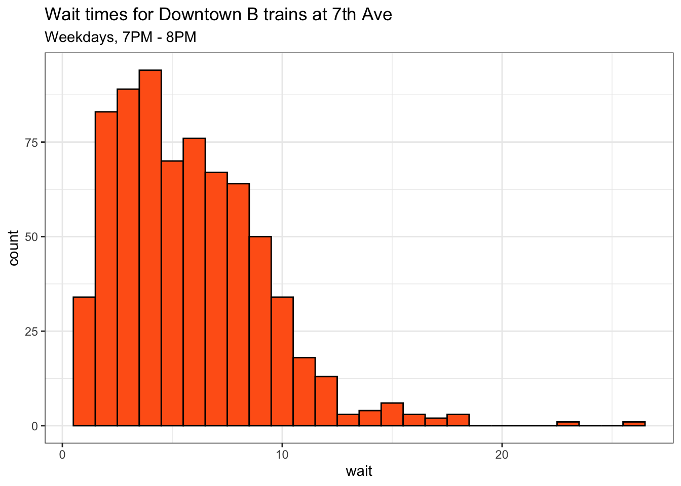
Is that little second bump enough to flip the relationship between platform crowdedness and wait times? You could probably fit some sort of flexible density function to the above histogram and come up with an “exact” answer to that question. But it’s much more fun to simulate, and even more fun to visualize that simulation.

So let’s establish some rules for our simulation:

• there are short, exponential delays between each arriving passenger, which creates more or less a uniform incoming flow of people
• train delays are sampled from the empirical delays that created the bimodal distribution above
• when trains arrive they entirely clear the platform
• each passenger “remembers” how many people are on the platform when they arrive and how long it takes for the train to arrive
• once passengers board the train, those data points are recorded on a scatterplot

I brought this idea to life using the Javscript library D3. Most of the code was generated by my prompts to ChatGPT, as I actually have almost never created visualizations outside of R – if you’re curious, the entire script is hosted on Observable.

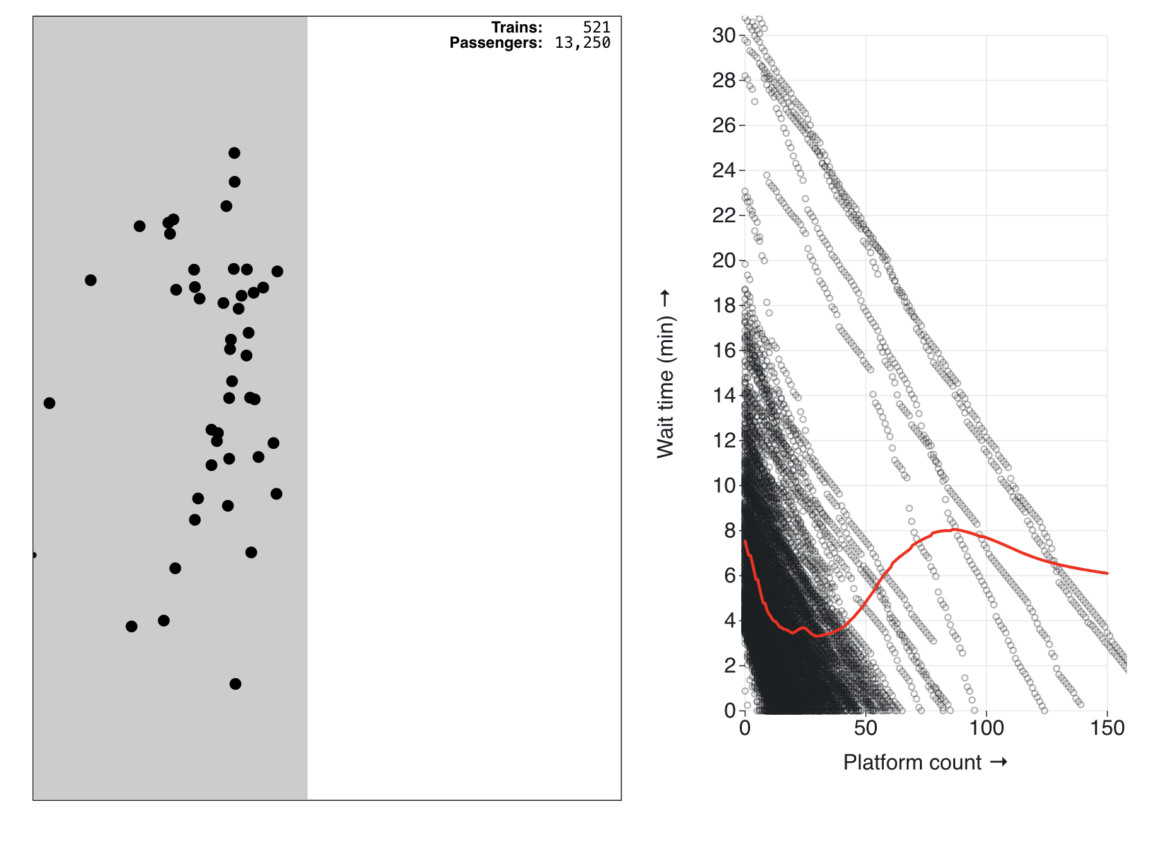
On the left, you’ll see passengers filter in continuously and spread out until a train appears from the top of the frame and whisks them away. Once the train has left, each passenger’s observed platform count and subsequent wait time is plotted on the graph to the right with an updating smoothed red trendline:

It does not take very many trains to establish the obvious pattern that describes most scenarios: as you increase the platform crowdedness from 0 to approximately 50, the average wait time for a train decreases.

However, if you let the simulation run long enough (sometimes it takes hundreds of trains), a sufficient number of extreme delays are sampled from that second mini-mode to create the “flipped” relationship that we’re looking for. A handful of trains fill in data for the large crowds (50+) further down the X-axis where there are otherwise very few points. The trendline bends up out there, just as we had hypothesized, as the only time the platform gets that crowded is when these delayed trains cause long wait times:

So according to a simplified model of a particular station at a specific time, yes it is possible that there’s such thing as “too many people” when you’re hoping for an imminent train. But overall I would not categorize these results as robust evidence of the phenomenon that I and many others assumed existed when it comes to subway delays.

library(archive)
library(tidyverse)
library(lubridate)
library(furrr)

# https://data.ny.gov/Transportation/MTA-Subway-Stations/39hk-dx4f/about_data
post_dir <- "/Users/walkerharrison/Documents/GH2/website/content/posts/2025-11-09-train-wait"
stations <- read_csv(paste0(post_dir, "/MTA_Subway_Stations_20251109.csv"))
stations_lite <- stations %>% transmute(stop_id = as.character(`GTFS Stop ID`), stop = `Stop Name`)

get_trains_by_date <- function(date){
  
  link <- paste0("https://subwaydata.nyc/data/subwaydatanyc_", date, "_csv.tar.xz")
  
  td <- tempdir()
  tf <- paste0(td, "\\tmp.tar.xz")
  
  download.file(link, tf)
  
  archive_extract(tf, td)
  allfiles <- list.files(td, full.names = T)
  stopfile <- allfiles %>% keep(~str_detect(.x, "stop_times"))
  tripfile <- allfiles %>% keep(~str_detect(.x, "trips"))
  
  stops <- read_csv(stopfile) %>% suppressWarnings() %>% suppressMessages()
  trips <- read_csv(tripfile) %>% suppressWarnings() %>% suppressMessages()
  
  stops <- stops %>% separate(stop_id, into = c("stop_id", "stop_id_direction"), sep = 3)
  trips <- trips %>% select(-last_observed, -marked_past)
  
  stops_clean <- stops %>% distinct() %>%
    inner_join(trips, by = "trip_uid") %>%
    mutate(departure_time = as.POSIXct(departure_time, origin="1970-01-01"),
           h = hour(departure_time),
           wd = wday(departure_time),
           weekend = !(wday(departure_time) %in% 2:6)
    ) %>%
    filter(as.Date(departure_time) == date) %>%
    select(trip_uid, route_id, direction_id, stop_id, track, arrival_time, departure_time, h, wd, weekend) %>%
    arrange(departure_time) %>%
    group_by(stop_id, route_id) %>%
    mutate(last_departure = lag(departure_time),
           wait = as.numeric(difftime(departure_time, last_departure, units = "secs"))/60) %>%
    filter(!is.na(wait), wait > 0) %>%
    ungroup() %>%
    mutate(route_id = as.character(route_id))
  
  file.remove(allfiles)
  
  stops_clean
  
}

dates <- seq.Date(from = as.Date("2025/1/1"), to = as.Date("2025/10/1"), by = "day")

stops <- get_trains_by_date(tail(dates, 1))

g1 <- stops %>%
  filter(route_id == "4", direction_id == "0", h >=9) %>%
  inner_join(stations_lite, by = "stop_id") %>%
  group_by(trip_uid) %>% 
  mutate(total_stops = n()) %>%
  filter(total_stops > 20, sum(stop_id == 250) > 0) %>%
  ungroup() %>%
  arrange(desc(total_stops), departure_time) %>% #View()
  mutate(stop = factor(stop, levels = unique(.$stop))) %>%
  # group_by(trip_uid) %>%
  # arrange(min(departure_time)) %>%
  # ungroup() %>%
  # filter(as.numeric(as.factor(trip_uid)) %in% 4:12) %>%
  {
  ggplot(., aes(departure_time, as.numeric(stop), group = trip_uid)) + 
  geom_point(col = "#01AB4F") + geom_line(col = "#01AB4F") +
  theme_minimal() +
  labs(x = "", y = "") +
  scale_y_continuous(breaks = 1:length(levels(.$stop)), labels = levels(.$stop))
  }

plan(multisession, workers =  4)

stops_all <- future_map(dates, get_trains_by_date) %>% bind_rows()

rush_hour <- stops_all %>%
  filter(h == 17, !weekend) %>%
  mutate(id = as.numeric(as.factor(paste0(route_id, direction_id, stop_id)))) %>%
  group_by(id) %>%
  mutate(n = n()) %>%
  ungroup() %>%
  mutate(n = n +  id/max(id)) %>%
  arrange(desc(n)) %>%
  group_by(route_id) %>%
  filter(stop_id == first(stop_id), direction_id == first(direction_id)) %>%
  ungroup() %>%
  filter(id %in% unique(.$id)[1:16]) %>%
  inner_join(stations_lite, by = "stop_id")

route_colors <- tribble(
  ~route_id, ~col,
  "1",  "#EC352F",
  "2",  "#EC352F",
  "3",  "#EC352F",
  "4",  "#01AB4F",
  "5",  "#01AB4F",
  "6",  "#01AB4F",
  "6X", "#01AB4F",
  "7",  "#B833AD",
  "7X", "#B833AD",
  "A",  "#2A51AE",
  "B",  "#FF6318",
  "C",  "#2A51AE",
  "D",  "#FF6318",
  "E",  "#2A51AE",
  "F",  "#FF6318",
  "G",  "#6CBD45",
  "J",  "#996633",
  "L",  "#A7A9AD",
  "M",  "#FF6318",
  "N",  "#FDCC0B",
  "Q",  "#FDCC0B",
  "R",  "#FDCC0B",
  "GS", "#808283",
  "W",  "#FDCC0B",
  "Z",  "#996633"
)

g2 <- rush_hour %>% 
  filter(wait > 1, wait < 15) %>%
  mutate(stop = str_replace(stop, " Bus Terminal", "")) %>%
  ggplot(aes(wait)) +
  geom_histogram(col = "black", aes(fill = route_id)) +
  theme_bw() +
  facet_wrap(~paste0(route_id, " at ", stop), scales = "free_y") +
  labs(title = "Rush hour wait distributions") +
  theme(legend.position = "none",
        strip.text.x = element_text(size = 7)) +
  scale_fill_manual(values = route_colors$col, breaks = route_colors$route_id)

downtown_Bs <- stops_all %>% filter(route_id == "B", direction_id == 1, stop_id == "D14", h == 19, !weekend)

g3 <- downtown_Bs %>%
  filter(wait > 1, wait < 30) %>%
  ggplot(aes(wait)) +
  geom_histogram(aes(fill = route_id), col = "black", binwidth = 1) +
  theme_bw() +
  labs(title = "Wait times for Downtown B trains at 7th Ave",
       subtitle = "Weekdays, 7PM - 8PM") +
  theme(legend.position = "none") +
  scale_fill_manual(values = route_colors$col, breaks = route_colors$route_id)

save(g1, g2, g3, file = paste0(post_dir, "/graphs.Rdata"))