
Many moons ago, when people actually physically went to work everyday, I had a pretty lengthy commute by New York City standards. Of the handful of ways to get from Park Slope, Brooklyn to my office in Yankee Stadium, I chose to take the 2/3 train from Grand Army Plaza and then transfer to the 4 train at Nevins Street for the remainder of the trip, typically clocking in at around an hour in travel time.
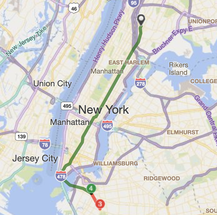
At some point though I started simply walking the first leg from my home to the Nevins Street station. That seems a little crazy, since I was substituting a few stops on the 2/3 for a mile-long march, but I enjoyed the exercise — and I also felt a little more relaxed once I got on the 4-train after my stroll.
Why did I find peace by walking the first part of my commute? Perhaps the exercise-induced endorphins were rushing through me by the time I was sitting on the 4-train. But I also wonder if I had accidentally decreased the variance in my commute time and with it some of the stress I feel wondering how long the my trip will take.
How? Well if we consider the duration of the full commute, \(X\), to be the sum of the two legs, \(Y_1\) and \(Y_2\), then the variance of the full commute would be the sums of the variances of the two legs, assuming that \(Y_1\) and \(Y_2\) are independent (which may not necessarily be the case, since subway routes are all a part of a coordinated network):
\[ X = Y_1 + Y_2; \ \ \ Y_1 \perp Y_2 \] \[ \text{Var}(X) = \text{Var}(Y_1) + \text{Var}(Y_2) \]
As a result, as long as my walks had less variance than the time spent waiting for and riding the 2/3 train until Nevins Street, then the overall variance would also be decreased, since the second leg is identical in both cases. Lucky for us, we can actually test this thought using some historical subway data.
Don’t like/know/care about R? Click here to skip to the results.
The MTA publishes the historical timestamp data of its subway routes, although there are some caveats. I was unable to successfully retrieve the “daily roll-up” files, which meant I had to grab the individual reports that correspond to 5-minute intervals. It also appears that the MTA stopped making these files available at some point in late 2018.
Either way, I’m able to fetch approximately 200 mornings’ worth of weekday data from 2018, which should suffice:
library(gtfsway)
library(httr)
library(tidyverse)
library(lubridate)
set.seed(0)

base_url <- "https://datamine-history.s3.amazonaws.com/gtfs"

date <- seq(ymd('2018-01-01'), ymd('2018-12-31'), by = 'days')

holidays <- as_date(c('2018-01-01', '2018-01-15', '2018-02-12', '2018-02-19',
                      '2018-05-28', '2018-07-04', '2018-09-03', '2018-11-12',
                      '2018-11-22', '2018-12-05', '2018-12-25'))

# all 2018 non-holiday weekdays
date <- date[!wday(date) %in% c(1, 7) & !date %in% holidays]

# all 5-minute intervals between 8 and 10 AM
hour <- 8:9 %>% str_pad(2, pad = "0")
minute <- seq(1, 56, by = 5) %>% str_pad(2, pad = "0")

urls <- crossing(date, hour, minute) %>%
  mutate(url = paste(base_url, date, hour, minute, sep = "-")) %>%
  pull(url)
Making this many queries to a somewhat unreliable data source requires some defensive programming, which is why the wrapper function safe_get waits a beat between runs and also won’t error if GET fails. A loop is used in place of something like map so as to not lose progress if the process gets hung somewhere and needs to be killed:
# pause between queries and fail gracefully
safe_get <- safely(function(url) {Sys.sleep(runif(1, 2, 3)); GET(url)})

requests <- list()

for(i in 1:length(urls)){
  requests[[i]] <- safe_get(urls[i])
}

# only keep the successful queries
good_requests <- requests %>%
  keep(function(request) !is.null(request$result$status_code) && request$result$status_code == 200)
The gtfsway package is a life-saver here since it converts the Google transit feed into comprehensible R objects, although I did rewrite the gtfs_tripUpdates function to drill down on specific routes in the interest of speed:
# slight re-write of gtfs_tripUpdates that runs faster
source("faster_trip_updates.R")

# station IDs corresponding to my commute
my_stops <- as.character(c(234:237, 414:423, 621, 626, 629, 631, 635, 640))

trip_updates <- imap_dfr(good_requests, function(request, idx){

  trip_updates <- request$result %>%
    gtfs_realtime() %>%
    # customized function that accepts routes
    gtfs_tripUpdates2(routes = as.character(2:4)) %>%
    imap_dfr(~cbind(
      idx = .y,
      url = request$result$url,
      .x$"dt_trip_info",
      .x$"dt_stop_time_update"
    ))

  # only return updates for my stops
  if(nrow(trip_updates > 0)){
    trip_updates <- trip_updates %>%
      separate(stop_id, into = c('stop_id', 'direction'), sep = "(?=[A-Z]$)") %>%
      filter(stop_id %in% my_stops)
  }

})
We again hit up the MTA developer site to pull in the station info, and then clean up our dataframe of trip updates so that the timestamps are formatted correctly:
stops <- read_csv('http://web.mta.info/developers/data/nyct/subway/Stations.csv') %>%
  janitor::clean_names() %>%
  select(gtfs_stop_id, stop_name, daytime_routes)

trip_updates <- trip_updates %>%
  inner_join(stops, by = c('stop_id' = 'gtfs_stop_id')) %>%
  mutate(dt = as_datetime(str_extract(url, '\\d{4}-\\d{2}-\\d{2}-\\d{2}-\\d{2}'), format = "%Y-%m-%d-%H-%M"),
         arrival_time = ifelse(arrival_time == 0, departure_time, arrival_time)) %>%
  mutate(arrival_time = as_datetime(arrival_time, tz = "America/New_York"),
date = date(arrival_time))dplyr magic. As is, the dataset consists of every update from every five-minute interval that we retrieved, so a single stop on a single subway trip could have dozens of rows of refreshed arrival estimates. What we need to do is filter for:
- only the latest possible information about each stop on each trip
- only the four stops that comprise the first leg
- only trips that left the first station between 8 AM and 10 AM (or were the first of the day after 10 AM)
# trip updates for 2/3 trains

first_leg <- trip_updates %>%
  filter(route_id %in% c("2", "3"), direction == "N", str_detect(daytime_routes, "[23]")) %>%
  mutate(trip_id = paste0(trip_id, "_", date)) %>%
  group_by(trip_id, stop_id) %>%
  # use latest possible update for each trip/stop
  filter(dt == max(dt)) %>%
  arrange(trip_id, arrival_time) %>%
  group_by(trip_id) %>%
  # only use the four stops that make up the first leg
  filter(sum(stop_name == "Grand Army Plaza") == 1,
         sum(stop_name == "Nevins St") == 1) %>%
  mutate(seq = row_number()) %>%
  filter(seq >= seq[which(stop_name == "Grand Army Plaza")],
         seq <= seq[which(stop_name == "Nevins St")]) %>%
  filter(n() == 4) %>%
  ungroup() %>%
  mutate(stop_name = factor(stop_name, levels = unique(.$stop_name)),
         stop_idx = as.numeric(stop_name)) %>%
  group_by(trip_id) %>%
  # record when train leaves first stop
  mutate(start_time = arrival_time[which.min(stop_idx)]) %>%
  ungroup() %>%
  # filter for 8AM - 10AM window (or just after)
  filter(hour(start_time) >= 8) %>%
  mutate(diff = ifelse(hour(start_time) < 10, Inf, start_time)) %>%
  filter(hour(start_time) < 10 | diff == min(diff)) %>%
  select(-diff) %>%
  mutate(route = "first leg (2/3)")
The logic for the second leg is similar, although now we have to record when exactly the first leg is finishing up each day, since these transfers will determine the window during which our second leg can actually start.
# find earliest and latest times when first leg is ending
transfers <- first_leg %>%
  filter(stop_idx == max(stop_idx)) %>%
  group_by(date) %>%
  summarize(first = min(arrival_time),
            last = max(arrival_time))

second_leg <- trip_updates %>%
  filter(route_id == "4", direction == "N", str_detect(daytime_routes, "4")) %>%
  mutate(trip_id = paste0(trip_id, "_", date)) %>%
  group_by(trip_id, stop_id) %>%
  # use latest possible update for each trip/stop
  filter(dt == max(dt)) %>%
  arrange(trip_id, arrival_time) %>%
  group_by(trip_id) %>%
  # only use the 14 stops that make up the second leg
  filter(sum(stop_name == "Nevins St") == 1,
         sum(stop_name == "161 St-Yankee Stadium") == 1) %>%
  mutate(seq = row_number()) %>%
  filter(seq >= seq[which(stop_name == "Nevins St")],
         seq <= seq[which(stop_name == "161 St-Yankee Stadium")]) %>%
  filter(n() == 14) %>%
  mutate(stop_name = factor(stop_name, levels = unique(.$stop_name)),
         stop_idx = as.numeric(stop_name) + max(first_leg$stop_idx) - 1) %>%
  inner_join(transfers, by = 'date') %>%
  # record when train leaves first stop
  mutate(start_time = arrival_time[which.min(stop_idx)]) %>%
  ungroup() %>%
  # filter for the transfer window (or just after)
  filter(start_time > first) %>%
  mutate(diff = ifelse(start_time < last, Inf, start_time - last)) %>%
  group_by(date) %>%
  filter(start_time < last | diff == min(diff)) %>%
  ungroup() %>%
  select(-first, -last, -diff) %>%
  mutate(route = "second leg (4)")
Put the two legs together and you get all the possible complete subway rides, transfers included, had I arrived at the first station (Grand Army Plaza) between 8 AM and 10 AM. Below are those rides for January 2nd, 2018:
full_trip <- rbind(first_leg, second_leg)

full_trip %>%
  filter(month(arrival_time) == 1, day(arrival_time) == 2) %>%
  arrange(desc(route)) %>%
  mutate(route = factor(route, levels = unique(.$route))) %>%
  ggplot(aes(arrival_time, stop_idx, group = trip_id)) +
  geom_line(aes(col = route)) +
  geom_point(aes(col = route), alpha = 0.5, size = 2) +
  scale_y_continuous(breaks = 1:max(full_trip$stop_idx),
                     labels = unique(c(levels(first_leg$stop_name), levels(second_leg$stop_name)))) +
  labs(x = "time", y = "") +
  facet_wrap(~date(arrival_time), scales = "free_x", nrow = 1) +
  theme_bw() +
  theme(legend.title = element_blank(),
        legend.position = c(1, 0),
        legend.justification = c(1, 0),
        legend.background = element_rect(fill = alpha("white", 0)),
        legend.key = element_rect(fill = alpha("white", 0)),
        legend.margin=margin(r = 10, b = 15))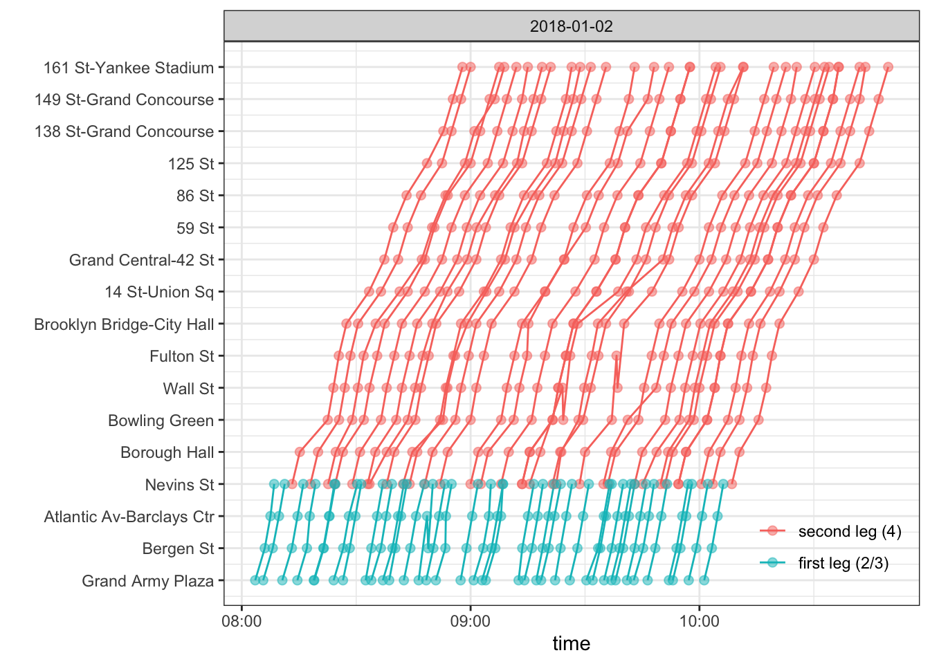
Don’t like/know/care about R? Click here to skip to the (other) results.
In order to use this data to estimate the distribution of the duration of the first leg, I need to simulate my arrival to Grand Army Plaza and calculate how long I’d have to wait to get on a train. To do so, I sample uniformly from the 8AM - 10AM window thousands of times across the various dates in the dataset and determine the first train I would have been able to board in each case:
# get duration of every possible first leg
two_three_trips <- full_trip %>%
  filter(route_id %in% c("2", "3")) %>%
  group_by(date, trip_id) %>%
  summarize(start = min(arrival_time),
            end = max(arrival_time))

n_sims <- 10000

# simulate arriving at station and taking first possible train
first_leg_subway <- data.frame(
  # random date, random time in morning
  date = sample(unique(transfers$date), n_sims, replace = TRUE),
  seconds_past_8 = runif(n_sims, 0, 60*60*2)
) %>%
  mutate(sim_idx = row_number()) %>%
  mutate(datetime = make_datetime(year(date), month(date), day(date),
                                  8, 0, seconds_past_8,
                                  tz = "America/New_York")) %>%
  inner_join(two_three_trips, by = 'date')  %>%
  filter(datetime < start) %>%
  group_by(sim_idx) %>%
  # find first train and calculate total commute time
  filter((start - datetime) == min(start - datetime)) %>%
  mutate(duration_leg1 = as.numeric(difftime(end, datetime, units = 'mins')))
Simulating the duration of my walk skews much more toward guesswork, since I don’t have actual daily data on how long it took each time. But I did recently time four walks down to Nevins and got pretty consistent times: 14:53, 15:05, 14:39, and 15:32. It feels reasonable to model the journey as normally distributed around 15 minutes with a standard deviation of 30 seconds. (It’s also entertaining to imagine what would have to happen to explain the fraction of walks that would theoretically take 20+ minutes – chased by a street gang in the wrong direction?)
# simulating leaving house between 8 and 9:30 and then taking a N(15, 0.5) walk
first_leg_walking <- data.frame(
  date = sample(unique(transfers$date), n_sims, replace = TRUE),
  leaving_time = runif(n_sims, 0, 60*60*1.5),
  duration_leg1 = rnorm(n_sims, mean = 15, sd = 0.5)) %>%
  mutate(sim_idx = row_number()) %>%
  mutate(end = make_datetime(year(date), month(date), day(date),
                             8, 0, leaving_time + 60*duration_leg1,
                             tz = "America/New_York"))
Once we’ve simulated both versions of the first leg, we can just attach each one to the second leg data and determine which 4-train these hypothetical commuters would be able to board:
# get duration of every possible second leg
four_trips <- full_trip %>%
  filter(route_id %in% c("4")) %>%
  group_by(date, trip_id) %>%
  summarize(start = min(arrival_time),
            end = max(arrival_time))

# determine which 4-train simulated subway commuters could board
full_trip_subway <- first_leg_subway %>%
  inner_join(four_trips, by = 'date', suffix = c("_leg1", "_leg2")) %>%
  filter(end_leg1 < start_leg2) %>%
  group_by(sim_idx) %>%
  filter(start_leg2 == min(start_leg2)) %>%
  mutate(duration_full = as.numeric(difftime(end_leg2, datetime, units = 'mins')))

# determine which 4-train simulated walking commuters could board
full_trip_walking <- first_leg_walking %>%
  inner_join(four_trips, by = 'date', suffix = c("_leg1", "_leg2")) %>%
  filter(end_leg1 < start) %>%
  group_by(sim_idx) %>%
  filter((start) == min(start)) %>%
  mutate(duration_full = as.numeric(difftime(end_leg2, end_leg1, units = 'mins')) + duration_leg1)
Finally we can graph the distribution of simulated first leg and full commute durations under both conditions. As we guaranteed by assuming a relatively consistent walking time, the variance of the first leg is much wider when taking the train despite also having a much smaller mean. This discrepancy is passed along to the full commute durations, as there’s also less overall variance when walking the first leg:
commute_times <- rbind(
  full_trip_subway %>%
    ungroup() %>%
    select(duration_leg1, duration_full) %>%
    mutate(type = "first leg on subway"),
  full_trip_walking %>%
    ungroup() %>%
    select(duration_leg1, duration_full) %>%
    mutate(type = "first leg walking")
) %>%
  mutate(idx = row_number()) %>%
  gather(interval, duration, -idx, -type) %>%
  mutate(interval = ifelse(interval == "duration_leg1", "first leg", "full commute"))

commute_stats <- commute_times %>%
  group_by(type, interval) %>%
  summarize(mean = mean(duration), variance = var(duration)) %>%
  mutate(text = paste0("mean: ", round(mean, 2), "\n", "variance: ", round(variance, 2)))

commute_times %>%
  ggplot(aes(duration)) +
  geom_histogram(aes(fill = type), col = "black") +
  geom_label(
    data = commute_stats,
    size = 3,
    fill = "#F6F6F6",
    mapping = aes(x = c(40, 110, 40, 110), y = 6000, label = text),
    hjust = 1,
    fontface = "italic") +
  facet_grid(type~interval, scales = "free_x") +
  labs(x = "duration (minutes)") +
  theme_bw() +
  theme(legend.title = element_blank(),
        strip.text.y = element_blank())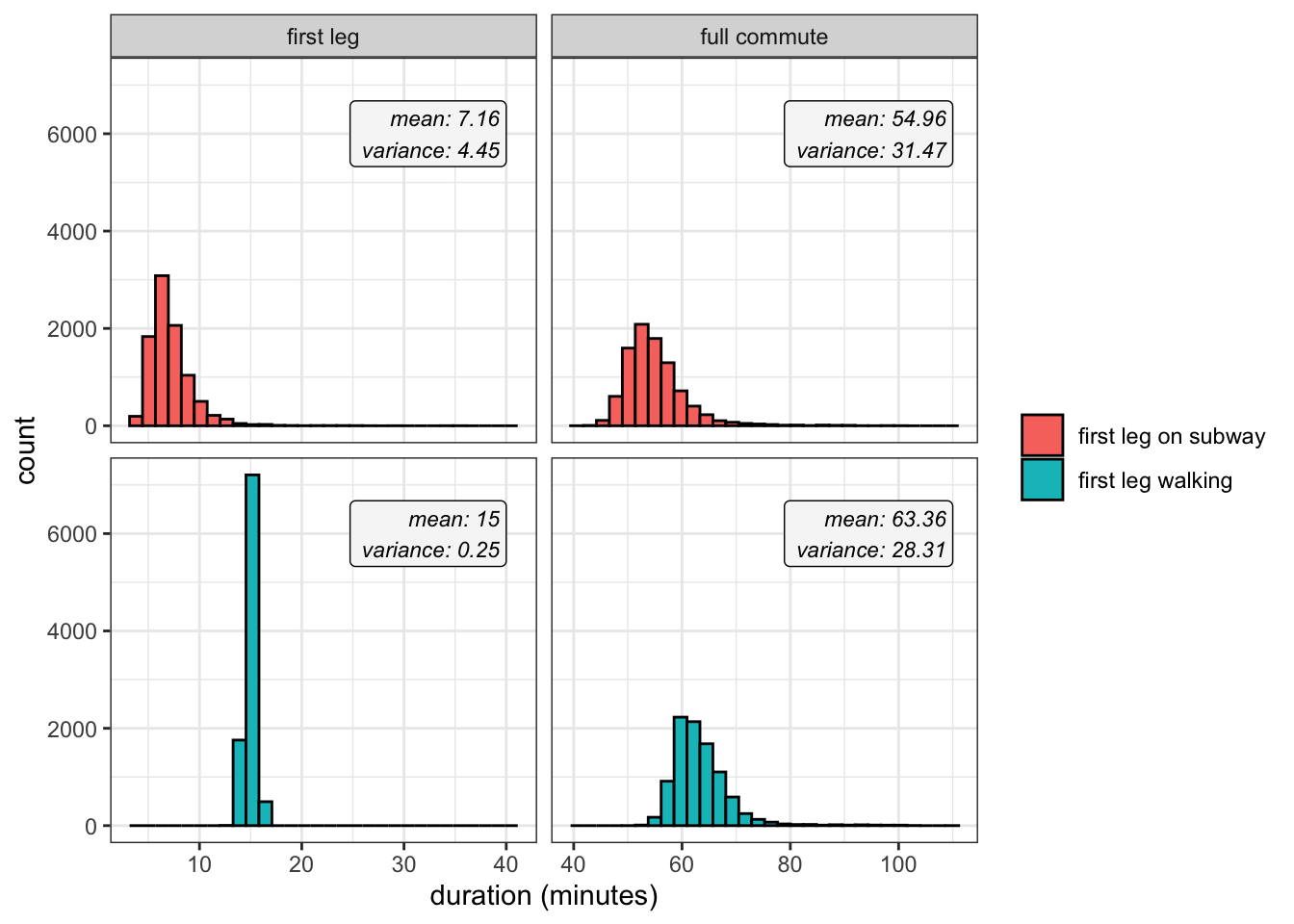
Of course, the two distributions describing the full journey are very similar, and the difference in spread is mostly washed away against the backdrop of lengthy commutes in general. By walking I wasn’t really saving that much uncertainty or avoiding particularly long trips that are usually caused by 4-train delays. But the study is still a decent example of a tradeoff between expected value and variance, which perhaps can explain why I found those walks a little more relaxing than waiting for a train.